Page 36 - 2024S

UEC Int’l Mini-Conference No.52 29

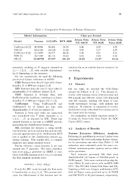
Table 1: Comparative Performance of Feature Extractors

Model Information Clips per Second

Jetson Orin Jetson Orin Jetson Orin
Model Params GFLOPs RTX 3090
NX 16GB NX 8GB Nano 8GB
UniFormer-B [9] 49.608M 64.202 31.50 2.42 2.09 1.63
C3D [6] 61.214M 154.120 34.22 3.68 3.17 2.67
UniFormer-S [9] 21.195M 28.717 66.08 5.40 4.64 3.54
TSM [7] 23.715M 66.110 85.42 8.64 7.59 6.04
I3D [5] 12.697M 27.877 101.23 16.92 15.27 11.34

extracted, resulting in N snippets denoted as termines the most suitable feature extractor for
f i , i = 1, 2, 3, . . . , N, with variable dimensional- our setting.
ity D depending on the extractor.
For our experiments, we used the following
pre-trained feature extractors in wVAD: 4 Experiments
C3D: Features from the fc6 layer with dimen- 4.1 Dataset
sionality D of 4096 per snippet [1,9].
I3D: Features from the mix 5c layer with di- For our tests, we selected the UCF-Crime
mensionality D of 1024 per snippet [2,3]. dataset by Sultani et al. [1]. This dataset in-
TSM: Adjusted to 16-frame clips, with cludes 1,610 training videos (810 abnormal and
ResNet50 as the backbone, resulting in a dimen- 800 normal) and 290 test videos (140 abnormal
sionality D of 2048 per snippet [10,11,13]. and 150 normal), totaling 128 hours of real-
UniFormer: Using UniFormer-B and world surveillance footage, both indoors and
UniFormer-S for 16 frames per clip, with outdoors. It contains 13 categories of anoma-
dimensionality D of 512 per snippet [4]. lies labeled at the video level for training and at
Features f i from each video are segmented the frame level for testing.
and normalized into T static segments x i = For evaluation, we follow previous works [1–
1, 2, 3, . . . , T, as required by MIL. These seg- 4] using the frame-level Area Under the ROC
mented features x i are sent to a BERT module, Curve (AUC) metric.
generating the classification feature y cls .
MIL processes the features x i using specific 4.2 Analysis of Results
loss functions, such as ranking loss and smooth-
ness and sparsity terms [1,2]. Additionally, BCE Feature Extractor Efficiency Analysis:
Following the guidelines in section 3, initial tests
loss is applied to the classification feature y cls
during training. This enables MIL to evaluate determined the best-performing feature extrac-
segments and assign anomaly scores. tor for processing raw video clips (Table 1). All
During inference, input features f i are seg- extractors were evaluated under the same con-
mented into T segments. The video classifica- ditions: maximum power capacity and no other
tion score p(ˆy cls ), predicted by BERT, is com- active processes.
bined with MIL segment scores s(x i ) to calculate Each extractor processed 500 clips sized
the final segment anomaly score: 16x3x224x224 (16 frames of 224x224 pixels in
RGB format). Tests were conducted on edge de-
score(x i ) = s(x i ) · p(ˆy cls ) vices (Table 2) and a server with an RTX 3090
GPU. The NVIDIA Jetson Orin Nano and NX,
If only the MIL model is used, the final score featuring a 1024-core Ampere architecture GPU
is based solely on s(x i ) [1,2]. This process eval- with 32 Tensor cores, provided up to 40 TOPS
uates the effectiveness of the features and de- and 100 TOPS of AI performance, respectively.