Page 51 - 2024F

44 UEC Int’l Mini-Conference No.53

53rd UEC International Mini-Conference, 3rd~4th March, 2025, The University of Electro-Communications, Chofu, Tokyo, Japan
Interferometric Evaluation of Stokes Camera
*Akter MONIA 1,2 , Yoko MIYAMOTO 1,2
1 Department of Engineering Science, the University of Electro-Communications
2 Institute for Advanced Science, the University of Electro-Communications
1-5-1 Chofugaoka, Chofu, Tokyo, 182-8585, Japan
*Email: a2443014@edu.cc.uec.ac.jp
Keywords: Stokes parameter, Stokes camera, interferometer, spatial resolution, polarization fringes.
Introduction
Stokes parameter and Stokes Camera:
• The Stokes parameters are a set of values that describe the polarization state of an S 0 = I H + I V
electromagnetic oscillation. S 1 = I H − I V (1)
• A Stokes camera measures the polarization state as a function of position by combining intensity S 2 = I RD − I LD
distributions recorded under different polarization analyzer settings. S 3 = I RC − I LC
• To determine the Stokes parameters, at least four polarization components are required.
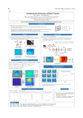
Objective Optical setup
Evaluation of the spatial resolution of Stokes camera: Generation of polarization fringes:
• To evaluate the spatial resolution of the Stokes camera (Photonic • The interferometer is used to create variations of polarization states
Lattice WPI 200) using Fourier analysis. with different spatial frequencies, and contrast in recorded Stokes
parameters is measured.
[HWP = Half Wave Plate, BS = Beam Splitter,
QWP = Quarter Wave Plate, M = Mirror]

Polarization Stokes camera: WPI-200
interferometer

Interferometer
Analysis using Recorded Stokes parameters
Fourier transform with fringe structure
S1 S1
Fourier Analysis
Left Right
∗
g x,y = a x,y + c x,y exp 2πi f x 0 x + f y0 y + x,y exp −2πi f x 0 x + f y 0 y 2 Circular Circular
Interferograms
∗
G f X ,f Y = A(f X ,f Y )+C(f X − f x 0 ,f Y − f y 0 )+ C (−f X − f x 0 ,−f Y − f y 0 ) 3
′ 4
G f X , f Y = C f X − f x0 , f Y − f y0 H f X − f x0 , f Y − f y0 Hann window filter and
′
ℱ −1 G f X , f Y = c x, y ∗ h x, y (5) tuning filter width
Contrast, b(x, y) =2|c(x, y)| (6)

−2
The maximum amplitude saturates at filter width 21x21 L , then
increases again due to noise.
|G f X ,f Y | |c x,y ∗ h x,y |
Result Evaluation Conclusion
Contrast vs Spatial Frequency Graph:
Interference between diagonally polarized beams: Interference between circularly polarized beams:
➢ The contrast is decreasing beyond spatial
frequency 0.20 pixel⁻¹ for interference between
diagonally polarized light.
➢ The contrast is gradually decreasing within
the frequency range of 0.04 to 0.12 pixel⁻¹.

S1 S3 S1 S2
References:
[1] S. Nagai, M. Akter, and Y. Miyamoto, Optical Manipulations and Structured Materials Conference 2024.
[2] M. Akter, S. Nagai, and Y. Miyamoto, Joint Symposia on Optics, Optics and Photonics Japan 2024.
[3] M. Takeda, H. Ina, and S. Kobayashi, J. Opt. Soc. Am.72 (1982) 156.