Page 12 - 2024F

UEC Int’l Mini-Conference No.53 5

The fundamental frequency (positive frequency
component) C(f − f 0 , y) is shifted to the cen-
ter of the spectrum to obtain C(f, y). Then,
the inverse Fourier transform of C(f, y) with re-
spect to f is computed to obtain c(x, y). The
fringe information can be obtained by inverse
Fourier transform of the fundamental frequency
information of the deformed fringe, as shown in
Equation 5:

1
log[c(x, y)] = log b(x, y) + iϕ(x, y) (5)
2
2.2 Unwrapping phase

Because in most cases, the computer-generated
phase main refers to the range from −π to π.
As shown in Figure 2 [11], the resulting wrap-
ping phase needs to be unwrapped.Therefore, Figure 2: (A) Example of a phase distribu-
the wrapped phase distribution is: tion having discontinuities that are due to the
principal-value calculation; (B) offset phase dis-

Im[c(x, y)] tribution for correcting the discontinuities in
ϕ(x, y) = arctan ,
Re[c(x, y)] (A); (C) continued profile of the phase distri-
ϕ(x, y) ∈ [−π, π] (6) bution. The y axis is normal to the figure.

If ϕ i+1 (x, y) − ϕ i (x, y) ≤ 0.9 × (−2π), then:
2.3 Gamma correction
ϕ i+1 (x, y) = ϕ i+1 (x, y)+2π, i = 0, 1, . . . , N−1. With the appearance of DLP with computer in-
terface and the decrease of price, it is increas-
If ϕ i+1 (x, y) − ϕ i (x, y) ≥ 0.9 × (2π), then:
ingly used in projection profilometry. How-
ever, due to the limitations of the equipment it-
ϕ i+1 (x, y) = ϕ i+1 (x, y)−2π, i = 0, 1, . . . , N−1.
self, the measurement accuracy will be reduced
due to nonlinear effects in the process of pro-
ducing fringes. In FTP, the normalized sinu-
One complete cycle (a phase change of 2π)
corresponds to a surface height change of one soidal fringes generated by computer program-
wavelength (λ). Thus, the relationship between ming and sent to DLP can be expressed as:
height h(x, y) and phase difference is given by:
u(x, y) = c + d cos(2πf 0 x + φ 0 (x, y)) (9)
λ
h(x, y) = ϕ(x, y), (7) c and d are the background and contrast of the
4π
fringes, respectively. Let φ 0 (x, y) = 0, then
where λ is the wavelength and ϕ(x, y) is the u(x, y) satisfies 0 ≤ (c−d) ≤ u(x) ≤ (c+d) ≤ 1.
phase difference. The two-dimensional Fourier Due to the nonlinearity of DLP, the output
transform of the function g(x,y): fringes of DLP are:
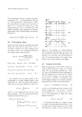
F(h(x, y)) =F(a(x, y))+ z(x, y) = [u(x, y)] γ (10)
1
F b(x, y)e iϕ(x,y) (u − f 0 , v)+ γ is generally not equal to 1. Figure 3 shows
2
1 the output (one-dimensional distribution) of si-
F b(x, y)e −iϕ(x,y) (u + f 0 , v) nusoidal input fringes passing through a DLP
2
(8) with different γ values. It can be seen that the