Page 15 - 2024F

8 UEC Int’l Mini-Conference No.53

Figure 9: Mask.

those simulated in matlab, we will not go into
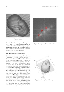
details here. The three-dimensional modeling Figure 10: Frequency domain information.
obtained through the final unwrapping opera-
tion is shown in Figure 11. You can see that the
surface of the model is not smooth, and there
are differences with the real model.

3.3 Experimental verification

An actual measurement was performed on a
”Face model.” The distances from the DLP to
the reference plane and CCD were L 0 = 780 mm
and d 0 = 240 mm, respectively. The period of
the sinusoidal grating was T 0 = 1/f 0 = 16 pix-
els, with c = d = 0.5. The construction of the
H(I) ∼ γ curve for the DLP and the gamma
value lookup followed the method in Section 1.2.
To improve the accuracy of γ, multiple refer-
ence fringes were collected in the experiment,
with each frame being calculated, and the final
value was taken as the average, representing the
DLP’s gamma value. In our experiment, we ob-
tained γ = 2.1531. After gamma correction us-
ing equation (12), FTP measurement was con-
ducted. The running time of gamma error com-
pensation is shown in Table 1 [13].The model re-
construction without gamma compensation and Figure 11: 3D modeling of the mask.
with gamma compensation is shown in Figure
12. Compared with the direct measurement
method without compensation, the time of the