Page 22 - 2024F

UEC Int’l Mini-Conference No.53 15

2P 3 = P 2 + P 4 . (2)
To construct an initial cubic Bézier spline that
1
satisfies C continuity, we can define the initial
control points that satisfies equation 2. Given a
sequence of points Q 0 , Q 1 , . . . , Q n that the spline
should pass through, each Bézier segment B i (t)
(i)
connects Q i and Q i+1 with control points P 1
and P (i) . The following is one way to initialize
2
(i) (i)
P 1 and P 2 ,
(i)
P 1 = Q i + α(Q i − Q i−1 ) (i > 0), (3)
P (i) = Q i+1 + α(Q i − Q i+1 ).
2
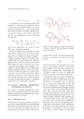
where α is a real number in the range (0, 1) and Figure 3: Bézier splines for same set with lower
(0) maximum curvature (up) and higher maximum
P 0 can be arbitrarily specified.
Equation 2 indicates that modifying a control curvature (down).
point affects only the curve itself and one adja-
cent curve to maintain continuity, giving cubic energy of the curve [5]. Curvature measures how
Bézier curves excellent local control properties. sharply a curve bends at a given point. It is de-
2
Higher continuity, such as C or above, is also fined as:
possible with more strict constraints. However, dθ
applying these constraint across an entire cubic κ = ds , (4)
Bézier spline will cause a cascading loss of local where θ is the angle of the tangent to the curve,
control over the tangent points, making it im- and s is the arc length. A larger curvature indi-
possible to edit the shape of curve while main- cates a sharper turn, while zero curvature cor-
taining continuity. Moreover, the visual “conti- responds to a straight line. Constraining the
nuity” is not entirely equivalent to mathematical maximum curvature of a curve is a simple way
continuity, and by utilizing additional degrees to make it smooth and aesthetically pleasing.
of freedom to achieve a lower maximum curva- The second factor is the node connection or-
ture, visually smoother curves can be obtained. der, which determines a sequence in which the
1
Therefore, in this study, we adopt C continuity points are connected. A poorly chosen sequence
constraints in the optimization algorithm.
can result in unnecessarily long or convoluted
curves, reducing the visualization quality. An
2.2 Factors Affecting Visualization effective approach is to compute the shortest
Performance in LineSets path that sequentially passes through all points
in the set, known as the shortest Hamiltonian
The quality of LineSets visualization is influ-
enced by several geometric factors, which can be path. This minimizes the path length while
broadly categorized into individual curve prop- avoiding self-intersections. For moderately sized
erties and multi-curve layout. data, the shortest Hamiltonian path can be effi-
ciently computed using the LKH algorithm [6].
The total length of the curve is also consid-
2.2.1 Individual Curve
ered. The curves obtained using the LKH algo-
For individual curves, the first factor is smooth- rithm and initial control points typically have a
ness, which requires that the curves should avoid length close to the shortest, while optimization
sharp turns and maintain natural flow. Smooth- of curvature and crossover layout may increase
ness can be quantified in multiple ways, such as the length. It is acceptable for the total length
measuring the maximum curvature or the strain of the curve to increase within a certain range