Page 24 - 2024F

UEC Int’l Mini-Conference No.53 17

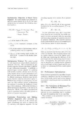
Optimization Objective of Each Curve preceding segment (if it exists), P is updated
′
2
Segment For a given Bézier curve segment de- as:
fined by control points P 0 , P 1 , P 2 , P 3 , the opti- P = 2P 0 − P 1 ,
′
2
mization aims to minimize the following objec-
tive function: where P 0 is the shared node of two segments.
Similarly, for the succeeding segment, P is up-
′′
1
dated to:
′′
f(P 1 , P 2 ) = w length · L + w curvature · K max P = 2P 3 − P 2 .
1
+ w intersections · N int (5)
In each optimization step, three consecutive
+ w angles · A penalty , curve segments are considered: the middle seg-
ment is actively optimized, while the preceding
where
and succeeding segments are passively adjusted
to maintain continuity. The objective function
• L is the length of the curve;
for the optimization is defined as a weighted sum
• K max is the maximum curvature of the of the function values for these segments:
curve;

• N int is the number of intersections, with in- F i = f i + 0.5f i−1 + 0.5f i+1 , 0 < i < n − 2, (6)
creased penalty near the endpoints;
where f i represents the function value f(P 1 , P 2 )
• A penalty is the crossing angle penalty, de- of the i-th segment. This weighting ensures that
fined as 90 −θ, where θ is the smaller cross- the middle segment receives the highest prior-
◦
ing angle. ity while also considering the influence of ad-
jacent segments for maintaining smooth transi-
Optimization Method The control points tions. Consequently, the optimization process
for each segment are independently adjusted to can be described as a sliding-window approach
minimize f(P 1 , P 2 ). The optimization is per- with a fixed length of three, improving the over-
formed using two different algorithms: L-BFGS- all shape by optimizing the local control points
B and Differential Evolution. L-BFGS-B, a in turn.
gradient-based method suitable for problems
with variable bounds, is chosen due to the rela- 2.5 Performance Optimization
tively smooth nature of most optimization vari-
ables and the small search space, which allows Using nonlinear optimization algorithms usually
for efficient convergence. However, since the ob- consumes a significant amount of computation
jective function contains non-convex parts, L- time. In this study, several methods are adopted
BFGS-B may converge to local optima. To mit- in geometric computing process to accelerate the
igate this risk, multiple random initializations algorithm.
are employed to increase the likelihood of find-
ing a better minimum. Differential Evolution, a 2.5.1 The Calculation of Maximum Cur-
global optimization algorithm, is also used as an vature of Bézier Curves
alternative. While it has higher computational
costs, it is preferred when a globally optimal so- The calculation of maximum curvature is a crit-
ical step in curve smoothing, and it consumes
lution is of greater importance.
the most of computing time in our algorithm.
The curvature at any parameter t can be cal-
Continuity Preservation and Sliding- culated as follows:
Window Approach After optimizing the
control points P 1 and P 2 of the current seg-
′
′′
′′
′
ment, adjustments are made to maintain the |B (t)B (t) − B (t)B (t)| (7)
y
x
y
x
C 1 -continuity with adjacent segments. For the κ(t) = (B (t) + B (t) ) ,
2
2 3/2
′
′
y
x